Data Analysis
Walk through a five-step workflow: import data, view descriptive statistics, check diagnostic plots, fit a statistical model, and run post-hoc comparisons.
Import Data
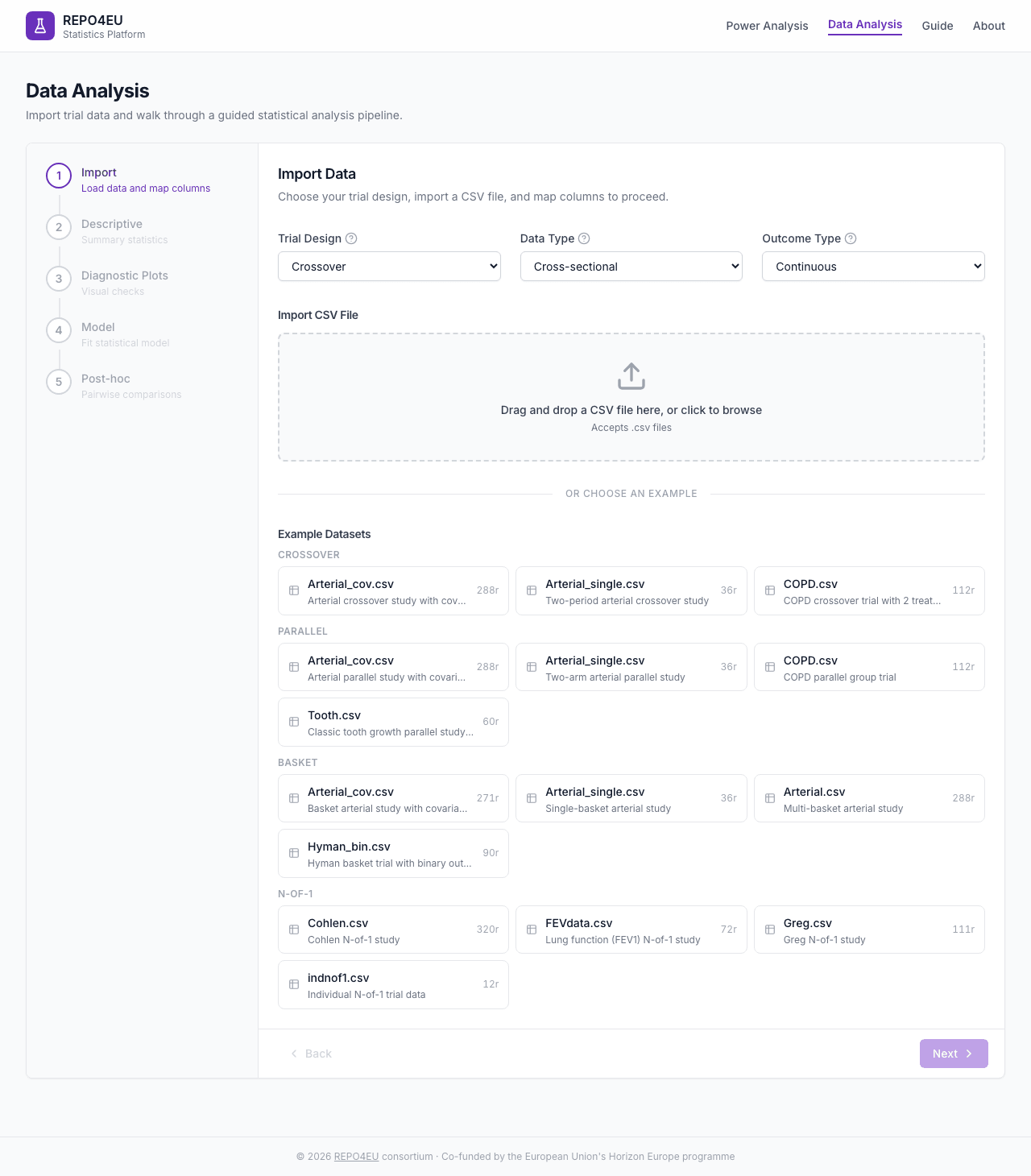
When the page loads, you see design selectors and a file import zone.

Initial state with design selectors and import area.
Design and Type Selectors
| Field | Description | Default |
|---|---|---|
| Trial Design | Crossover, Parallel, Basket, N-of-1, Umbrella | Crossover |
| Data Type | Cross-sectional, Longitudinal (crossover/parallel only) | |
| Outcome Type | Continuous, Binary | Continuous |
Loading Data
You can import a CSV via drag-and-drop, or choose from built-in example datasets.
Built-in example datasets including COPD crossover, arterial studies, and more.
After Import
Once data is loaded, a green badge confirms success with row/column counts and a data preview table.

Green badge confirms successful import with data preview.
Column Mapping
Map your data columns to the required roles: Response (Outcome), Treatment, Subject ID, and Period. Crossover data may also map Carryover; umbrella data maps Biomarker.
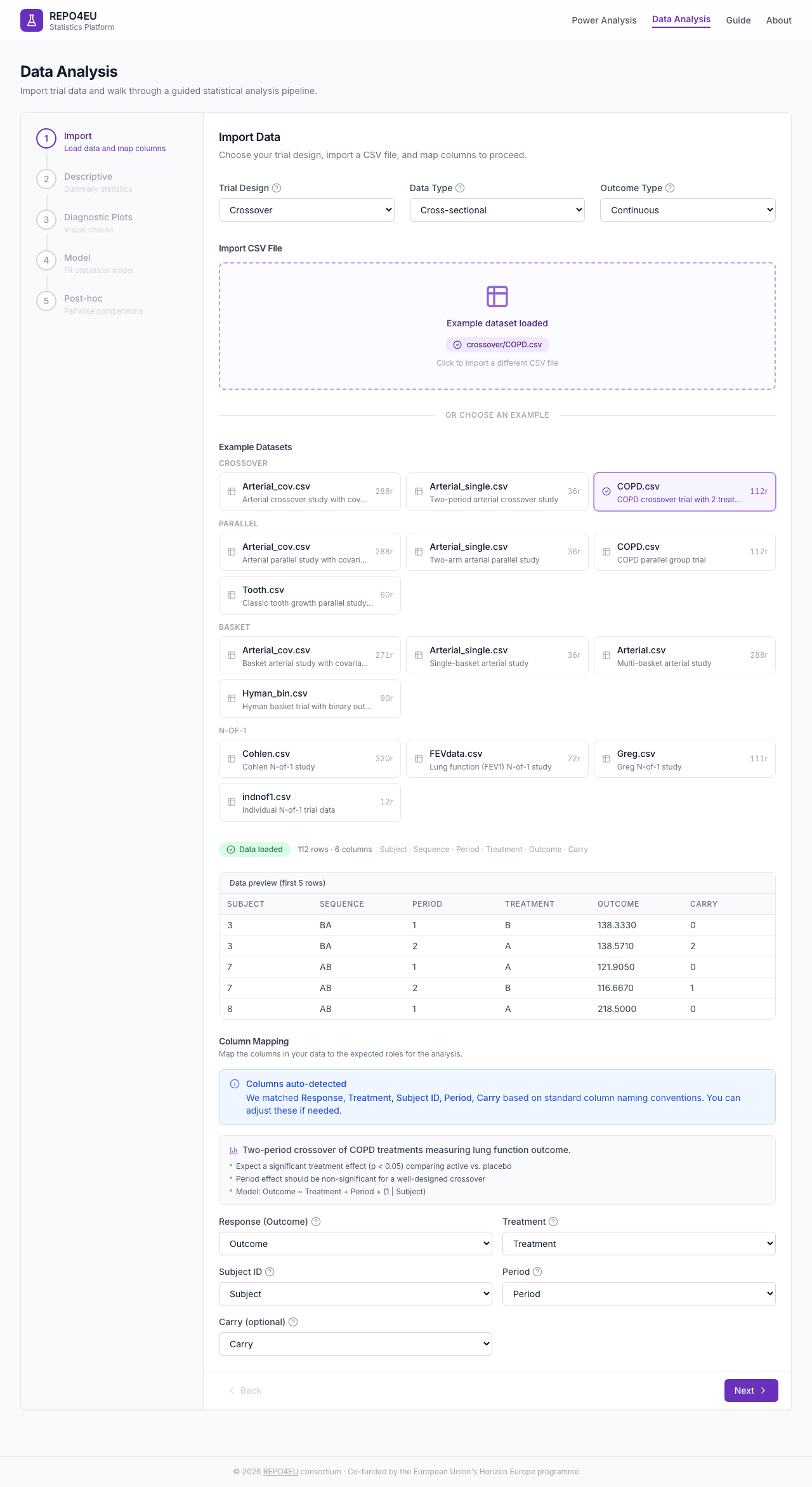
Map your CSV columns to the required roles.
Descriptive Statistics
Automatically computed when you enter this step. Includes participant flow, baseline characteristics, and outcome summary tables.
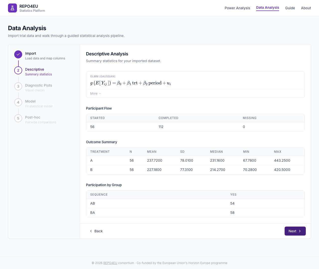
Participant flow, baseline characteristics, and outcome summary.
Diagnostic Plots
Select which plot types to generate: cross-sectional, longitudinal, profiles, or period. Plots are rendered as images from the R backend.
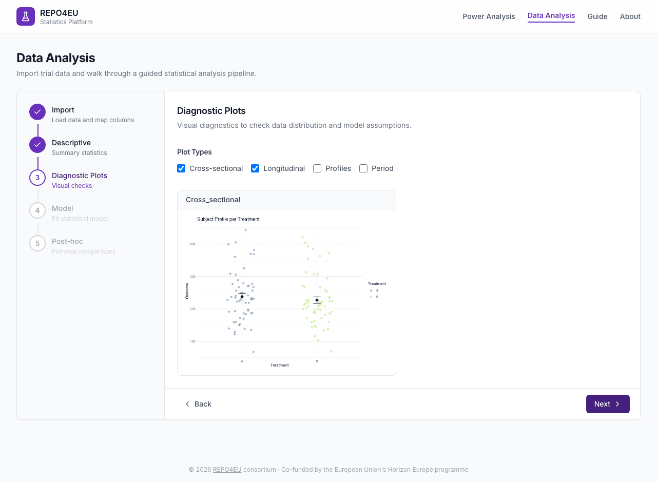
Visual diagnostics for model assumptions.
Reading residual plots
Look for points scattered randomly (good) in residual plots. Patterns, funnels, or clusters may indicate model assumption violations.Fit Model
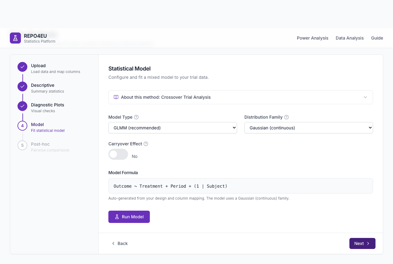
Configuration
| Field | Description | Default |
|---|---|---|
| Model Type | GLMM (recommended), GEE | GLMM |
| Carryover | Yes / No (crossover designs) | No |
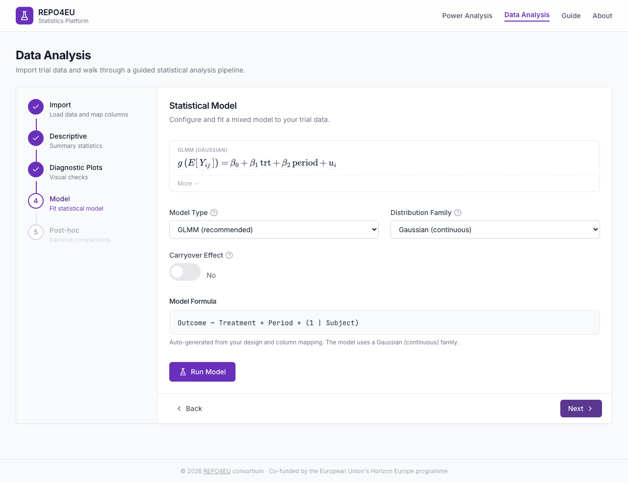
Select model type and options before fitting.
Results
After clicking Run Model, GLMM and GEE fits show coefficients and fit statistics. Basket models show posterior summaries; substudy-specific umbrella models show per-substudy drug-vs-control contrasts.
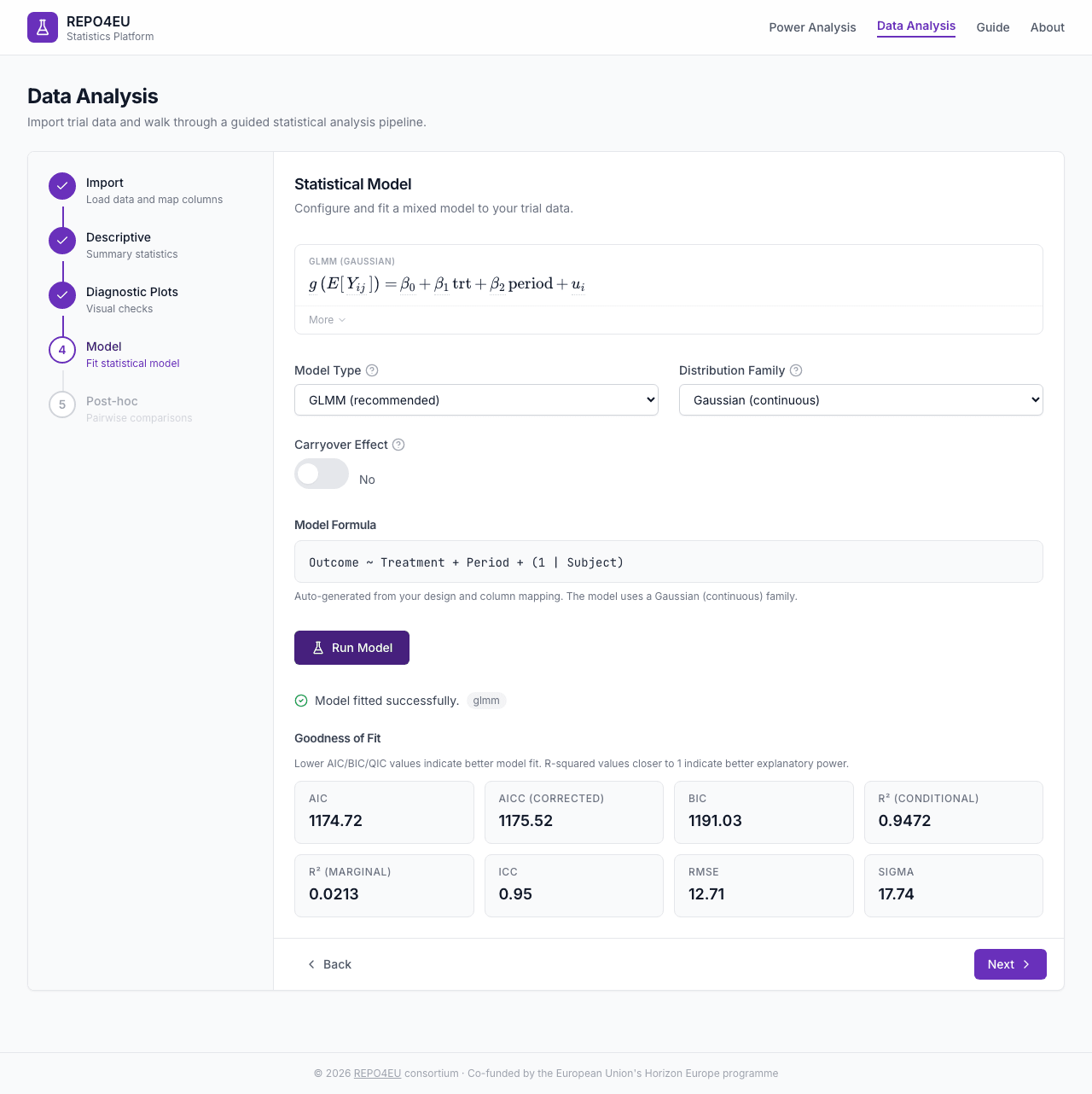
Coefficients table and model fit statistics.
Post-hoc Contrasts
Configuration
| Field | Description | Default |
|---|---|---|
| Factor | Model terms dropdown | |
| Contrast Type | Pairwise, Treatment vs Control, Custom Contrasts | Pairwise |
| P-Value Adjustment | None, Bonferroni, Holm, Tukey | None |
| Side | Two-sided, Greater, Less | Two-sided |
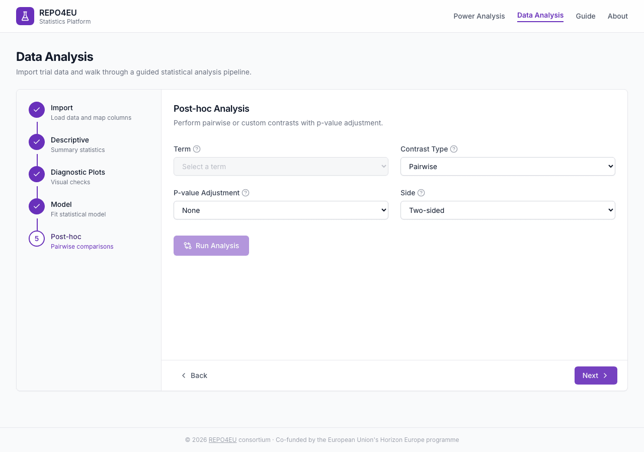
Configure contrast type and p-value adjustment.
Results
After clicking Run Post-hoc: estimated marginal means, contrasts table with p-values and confidence intervals, and EMM/contrast plots from R.
Estimated marginal means, contrasts, and plots.
P-value adjustment
When making multiple comparisons, use Bonferroni (simple), Holm (slightly more powerful), or Tukey (designed for pairwise). Use “None” only for a single pre-specified comparison.Concepts
Data Preparation
Import a CSV file with one row per observation. The platform expects columns for the response variable, treatment group, subject ID, and (for crossover/longitudinal designs) a period column. Built-in example datasets let you explore the workflow before importing your own data.
Statistical Models
Toggle between GLMM and GEE to see subject-specific regression lines vs a single population-average line.
- GLMM
- Generalized Linear Mixed Model - accounts for both fixed effects (treatment, period) and random effects (patient-level variation). Recommended for most trial designs.
- GEE
- Generalized Estimating Equations - models population-average effects. More robust to misspecification of the correlation structure, but does not provide subject-level predictions.
Diagnostics
Select a pattern to see what good and problematic residuals look like in both plot types.
Diagnostic plots help you check whether model assumptions hold. Residual vs. fitted plots should show random scatter (no funnels or curves). QQ plots should follow the diagonal line. Violations may indicate the need for a different model or data transformation.
Post-hoc Comparisons
Adjust group means and see which comparisons reach significance under different correction methods.
- Pairwise
- Compares all pairs of treatment groups. Best when you have no pre-specified reference group.
- Control
- Compares each treatment against a selected reference control. This is more focused than all pairwise comparisons.
P-value adjustment (Bonferroni, Holm, Tukey) controls the family-wise error rate when making multiple comparisons.
Basket Models
Compare independent, BHM, and EXNEX borrowing behavior. EXNEX is available for binary outcomes only.
- BHM
- Bayesian Hierarchical Model - borrows strength across baskets, improving power when effects are similar.
- IND
- Independent model - fits each basket without borrowing information across baskets.
- EXNEX
- Exchangeability/non-exchangeability model - allows each basket to be either exchangeable or independent. It is currently available for binary outcomes only.
Bayesian Basics
Widen the prior SD to see the posterior follow the data; narrow it to see the prior dominate.
Bayesian methods combine prior beliefs with observed data to produce posterior distributions. In basket trial analyses, borrowing information across baskets can reduce standard errors when treatment effects are similar. Prior distributions are set automatically based on the selected borrowing method.